Collision Detection – GJK Part 3

Welcome to the final post on implementing the GJK. In the first post, we looked at some of the basics and described the algorithm in general terms. In the second post we looked at how the GJK is set up in the Dubious Engine. In this post we’re going to dig down into the lowest layer, where we build and maintain the Minkowski Simplex.

Let me set the stage from our last post. We were in a loop, trying to find a new Support Point and Support Vector. If a suitable candidate was found, the loop would end like this (not really, but close, the real code is here)

    simplex.push_back( support_point);
    bool collision_found = simplex.build();
    if (collision_found) {
        return true;
    }

So we’re going to be looking at the Minkowski_simplex in detail. Internally it basically holds 4 points (the code is a little bit more complicated for efficiency’s sake). Why 4 points? Remember that in 3D a simplex is a tetrahedron, which is a shape made of 4 points. Not all 4 points are in use at all times. The algorithm starts with a simple Line (ie 2 points). When a new Support Point is added, the simplex becomes a Triangle. Then another new Support Point turns it into a Tetrahedron. If that is not found to contain the origin, then a point is dropped and the simplex becomes a Triangle again. Let’s take a look at how it works.

The Minkowski_simplex::push_back function is trivial. If it were implemented with an actual std::vector it would literally be a call to std::vector::push_back. But what’s up with the build function?

std::tuple<bool, Math::Vector>
Minkowski_simplex::build()
{
    switch (m_size) {
    case 2:
        return build_2();
    case 3:
        return build_3();
    case 4:
        return build_4();
    default:
        throw std::runtime_error("Received simplex of incorrect size");
    }
}

As you can see, there are only three valid point counts, corresponding to the Line, Triangle, and Tetrahedron.
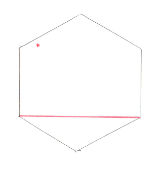
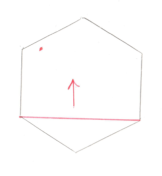
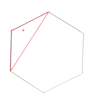
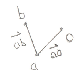
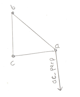
Test 1: Line

Given a simple Line of only two Points, this image shows the 3 possible areas where the origin could be:

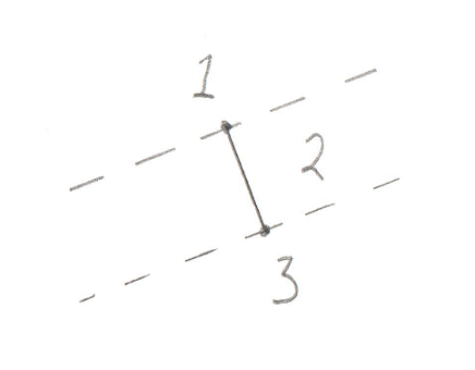
  1. Past the end of the Line
  2. Between the two ends of the Line
  3. Past the other end of the Line

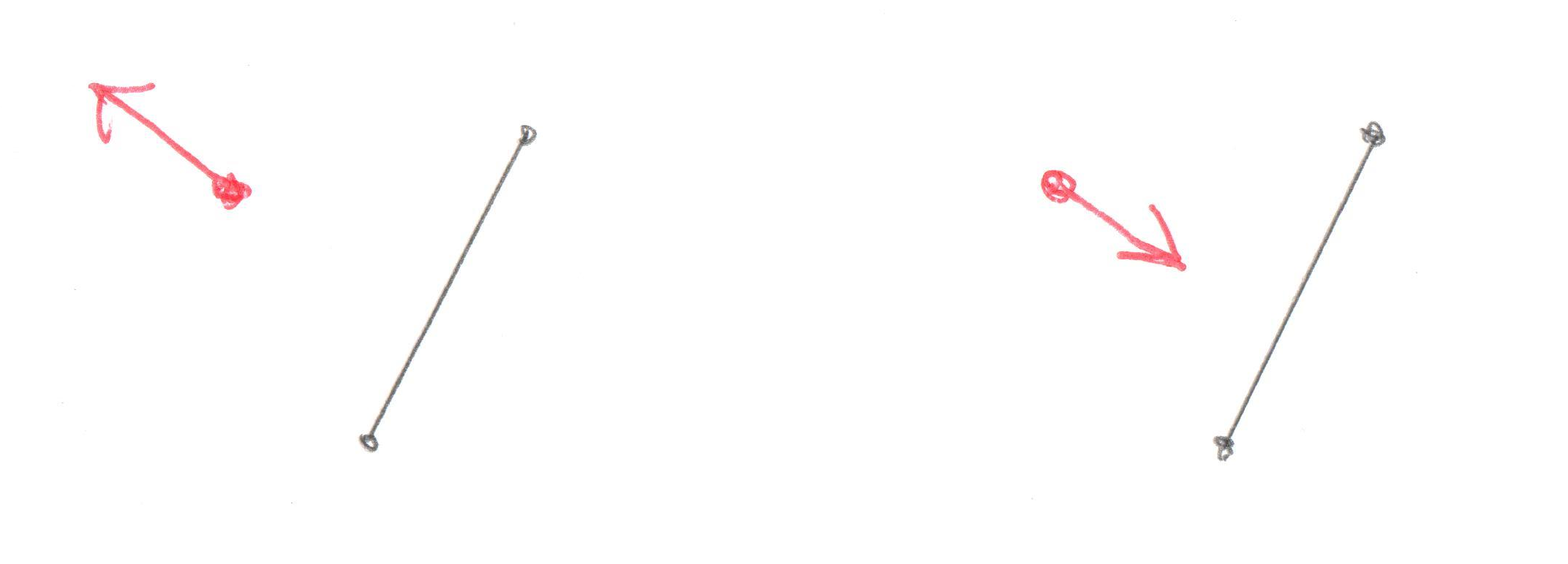
Hopefully that’s not too confusing. It turns out that there are actually less real possibilities. Recall in the previous post I devoted a lot of time to the dot_product test between the Support Point and Support Vector. I said it was “critically important.” The reason it’s so critical is that it lets us disregard areas 1 and 3 in the above image. This is because areas 1 and 3 correspond to a situation where the Support Point is out past the end of the Support Vector. And our dot_product test is done to look for exactly this situation, because if the Support Point is out past the end of the Support Vector then there’s no way the resulting simplex can contain the origin. To say it another way, the dot_product test has already filtered out areas 1 and 3, so we don’t even need to look for them. This makes the search for the origin in relation to this line very easy, the origin is either on one side or the other.

Let’s have a look at the code.

std::tuple<bool, Math::Vector>
Minkowski_simplex::build_2()
{
    const Math::Vector& a = m_v[1].v();
    const Math::Vector& b = m_v[0].v();
    const Math::Vector  origin;

    const Math::Vector& ab        = b - a;
    const Math::Vector& ao        = origin - a;

You’ll notice in all this code I try to name things consistently. Points in the simplex are a, b, c, and d, and the origin is o. A Vector pointing from a to b (counter-intuitively calculated by b-a) is called ab.

For this next bit I’m changing the real code by inserting a tmp Vector to make it a bit clearer

    Math::Vector        tmp = Math::cross_product(ab, ao);
    Math::Vector        direction = Math::cross_product( tmp, ab);

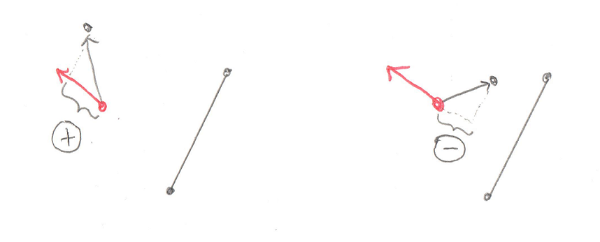
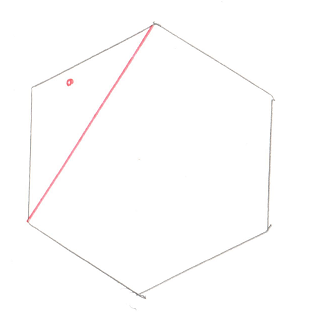
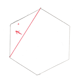
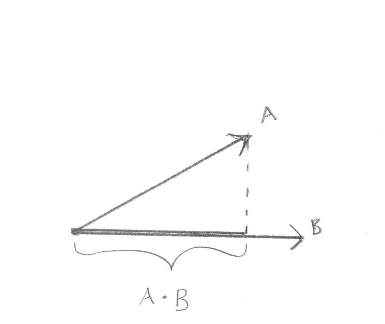
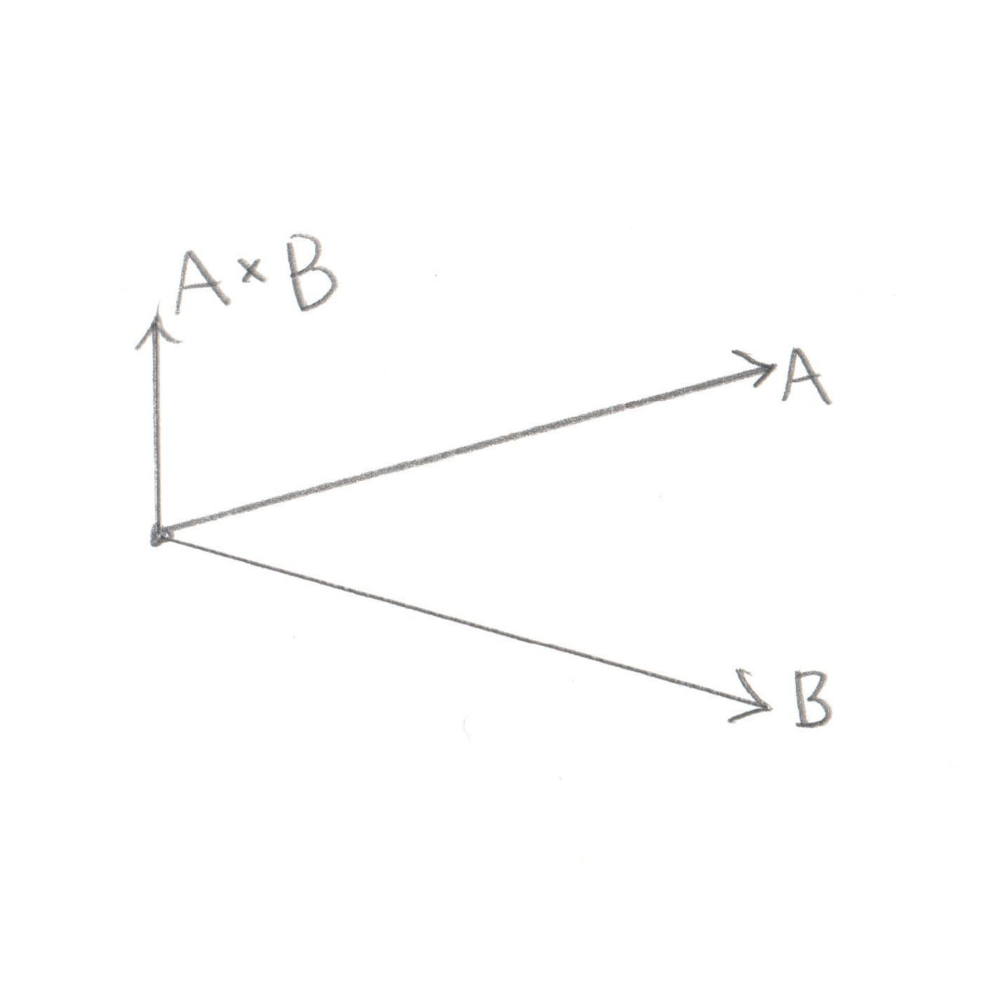
Okay, this is the important part of this test. Let’s look at what’s going on with these two Cross Products. What we’re trying to find is the direction of the origin. Let’s use this as an example, in this image we have Vectors ab and ao:

You’ll recall that a Cross Product of any two Vectors is a third Vector that is perpendicular to both of them. In this case the two Vectors both lie on the plane of your monitor, so the Cross Product of ab and ao, stored in tmp, is a new Vector that points directly out of your monitor and at you. Grab a pencil and stick the eraser on point a and point the tip at you, that’s the Vector tmp. The next part of the code takes the Cross Product of tmp and ab. That would be a new Vector that’s perpendicular to ab and points in the direction of the origin.

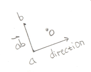
Pretty cool, huh? By using two Cross Products we’ve found the direction Vector we’re looking for. That will become the new Support Vector for the next phase of the GJK.

But before we move ahead, there’s an edge case to worry about (there’s always an edge case).

    if (direction == Math::Vector()) {
        if (Math::equals(fabs(ao.y()), 0) && 
            Math::equals(fabs(ao.x()), 0)) {
            direction = Math::Vector(0, 1, 0);
        }
        else {
            direction = Math::Vector(ao.y(), -ao.x(), 0);
        }
    }
    return std::make_tuple(false, direction);
}

If the origin happens to fall exactly on the Vector ab, then the Cross Product will fail and we’ll be left with an empty direction Vector. In this case we can try to create a perpendicular Vector manually.

So that’s the code for the Line test. Not too bad I hope. The following tests are basically the same idea, but with more possible locations to look for the origin, and a few quirks to deal with.
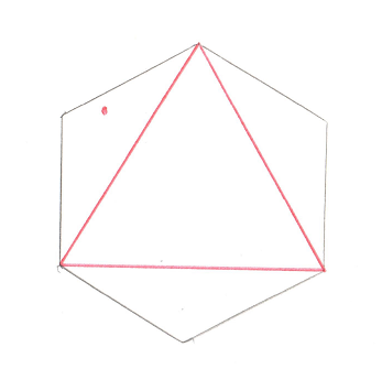
Test 2: Triangle

This one is a bit more complex, but it still breaks down into distinct places where the origin can be:

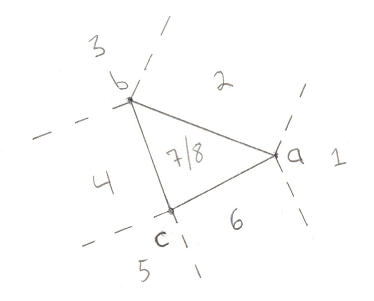
  1. Past Point A (not possible)
  2. Outside line AB
  3. Past Point B (not possible)
  4. Outside line BC (not possible)
  5. Past Point C (not possible)
  6. Outside line CA
  7. Above the triangle
  8. Below the triangle

We can eliminate cases 1, 3, and 5 due to the same optimization discussed for the Line test, if the origin was past the lines then we would give up before entering this test. We can also eliminate the outside of Vector bc. This is a bit of a surprise. This is because Vector bc turns out to be the Line we tested previously. In order to get to this stage we already know that the origin is on one side of Vector bc, so there’s no need to test the other side. What’s left is 2 Line tests (cases 2 and 6) and 2 Triangle tests (cases 7 and 8).

Let’s look at some code:

std::tuple<bool, Math::Vector>
Minkowski_simplex::build_3()
{
    const Math::Vector& a = m_v[2].v();
    const Math::Vector& b = m_v[1].v();
    const Math::Vector& c = m_v[0].v();
    const Math::Vector  origin;

    const Math::Vector& ab      = b - a;
    const Math::Vector& ac      = c - a;
    const Math::Vector& ao      = origin - a;
    const Math::Vector& ab_x_ac = Math::cross_product(ab, ac);

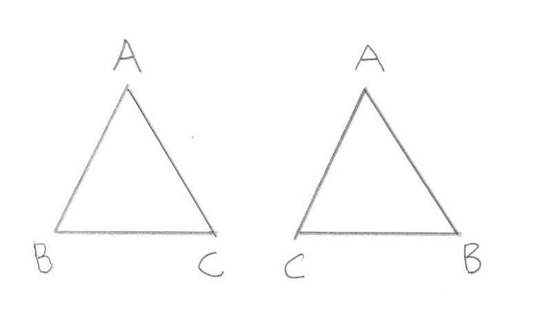
I discussed the naming of a, b, and c previously. It’s important to note that b and c are the same Points used in the above Line test. This is how we can exclude the test on the outside of bc. Vectors ab, ac, and ao are simply created by subtracting the points, same as last time. Vector ab_x_ac (pronounced “ab cross ac”) is the Triangle Normal, ie a Vector pointing perpendicular to the outside of the Triangle. Recall the discussion of the Winding Order, it’s very important that this Triangle is ABC and not ACB. You will see the code moving points around to make sure the winding remains consistent.

So what’s the plan of attack? For the lines tests (cases 2 and 6) we want to find a Vector that points away from an edge, and then test if the origin overlaps with that Vector. Let’s start with the ab edge:

    const Math::Vector& ab_perp = Math::cross_product(ab, ab_x_ac);
    if (Math::dot_product(ao, ab_perp) > 0) {
        m_v[0] = m_v[1];
        m_v[1] = m_v[2];
        --m_size;
        return std::make_tuple(false, ab_perp);
    }

The Vector ab_perp is a Vector perpendicular to edge ab.

Again we can use the Cross Product to find a Vector perpendicular to any two Vectors, in this case edge ab and the Triangle Normal. We can take the dot product of this new Vector and the ao Vector to find out if ao is on the outside of the Triangle along ab_perp. If it is then we throw away point c and reduce our Minkowski Simplex to a simple Line, and return a new Support Vector to search in.

If that test fails then we want to do the exact same test, but this time along edge ac:

    const Math::Vector& ac_perp = Math::cross_product(ab_x_ac, ac);
    if (Math::dot_product(ao, ac_perp) > 0) {
        m_v[1] = m_v[2];
        --m_size;
        return std::make_tuple(false, ac_perp);
    }

If this test passes then the origin is outside of the triangle on the ac side.

This means we have to throw away point b.

If none of these tests find the origin then we can conclude that it’s not outside of any of the edges, so it must be inside the Triangle. So now it’s just a question of whether the origin is above the triangle, or below it.

    float side_check = Math::dot_product(ab_x_ac, ao);
    if (side_check > 0) {
        return std::make_tuple(false, ab_x_ac);
    }

The check to see if it’s above the triangle is trivial, just use the Dot Product to see if Vector ao is along the Triangle Normal. If it is then we retain our entire Triangle and return the new Support Vector.

Finally if it’s not above our Triangle, it must be below it (okay fine, or precisely on it but that edge case doesn’t need to be handled differently)

    std::swap(m_v[0], m_v[1]);
    return std::make_tuple(false, ab_x_ac * -1);
}

Wait wait, what’s going on with the call to std::swap? Remember I said that the Winding Order is important? For our Tetrahedron test we need to know which side of the Triangle the origin is on. I set it up so that it’s always on the “outside.” But in this case, the origin is “inside” the Triangle. So I fix this by simply flipping two points on the Triangle, thereby reversing the Winding Order and making the old “inside” the new “outside.” Cool trick, huh?
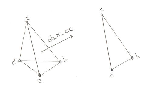
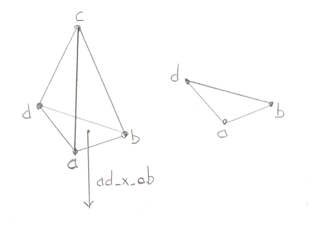
Test 3: Tetrahedron

Hoo boy, the Tetrahedron! If you’re comfortable with the triangle case then this one isn’t a stretch of the imagination. It is, however, a stretch of my drawing abilities:

For this image assume Point a is closest to you. Here’s the places where the origin could be:

  1. Past any of the 4 points (not possible)
  2. Outside triangle ABC
  3. Outside triangle ADB
  4. Outside triangle ACD
  5. Outside triangle BDC (not possible)
  6. Inside the Tetrahedron

I compressed the 4 end point checks into case 1. As before, they’re not possible in our situation due to the Dot Product test that I’ve been harping on about. And just like for the Triangle case it wasn’t possible to be outside of the Line we started with, for the Tetrahedron it’s not possible to be outside of the Triangle we started with (case 5).

Then there are 3 remaining triangle tests. If it turns out that the origin is outside of one of these Triangles then we drop the Point at the opposite side and are left with just a Triangle. Then we define the Support Vector to be in the direction from this Triangle to the origin. We grab a new Point and are left with a new Tetrahedron and the tests begin again.

Let’s bring on the code:

std::tuple<bool, Math::Vector>
Minkowski_simplex::build_4()
{
    const Math::Vector& a = m_v[3].v();
    const Math::Vector& b = m_v[2].v();
    const Math::Vector& c = m_v[1].v();
    const Math::Vector& d = m_v[0].v();
    const Math::Vector  origin;

    const Math::Vector& ab = b - a;
    const Math::Vector& ac = c - a;
    const Math::Vector& ad = d - a;
    const Math::Vector& ao = origin - a;

This bit should look very familiar by now. Let’s be very specific about the Winding Order. You’ll remember from the Triangle test above that we left with the Support Vector on the “outside” of the triangle. Since the new point would have been pushed back to the last position in the array, this means that points b, c, and d define the Triangle we were looking at before. This also means that a is “outside” the Triangle, and that from a‘s perspective, b, c, and d are wound counter-clockwise.

Next we set up the usual edge Vectors, ab, ac, ad, and the Vector to the origin, ao. We don’t bother defining the other edges (bc, bd, or cd) because we already know the origin can’t be outside of that Triangle (case 5 above) so there’s no need.

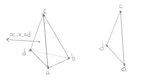
Let’s have a look at the test outside of Triangle ABC (case 2):

    const Math::Vector& ab_x_ac = Math::cross_product(ab, ac);
    if (Math::dot_product(ab_x_ac, ao) > 0) {
        m_v[0] = m_v[1];
        m_v[1] = m_v[2];
        m_v[2] = m_v[3];
        --m_size;
        return std::make_tuple(false, ab_x_ac);
    }

The Vector ab_x_ac (pronounced “ab cross ac”) is the Normal to Triangle ABC. By checking the Dot Product of that Normal with the Vector to the origin we can see if the origin is outside Triangle ABC. If it is then Triangle ABC becomes our new starting Triangle and ab_x_ac becomes out new Support Vector. This means we drop point d as we know the origin is not on that side of the Tetrahedron. Winding Order remains important as our next test needs to start off with the origin “outside” this Triangle.

There’s no need to dwell on the next two tests. They’re exactly the same, it’s just that the Triangles change. And again, if the origin is found to be outside then we have to be very careful of the Winding Order of the new Triangle that will be used for our next test. First here’s triangle ACD:

    const Math::Vector& ac_x_ad = Math::cross_product(ac, ad);
    if (Math::dot_product(ac_x_ad, ao) > 0) {
        m_v[2] = m_v[3];
        --m_size;
        return std::make_tuple(false, ac_x_ad);
    }

And lastly Triangle ADB:

    const Math::Vector& ad_x_ab = Math::cross_product(ad, ab);
    if (Math::dot_product(ad_x_ab, ao) > 0) {
        m_v[1] = m_v[0];
        m_v[0] = m_v[2];
        m_v[2] = m_v[3];
        --m_size;
        return std::make_tuple(false, ad_x_ab);
    }

And all of that work brings us to the final, glorious step in the GJK. If the origin is not outside of the 4 Triangles, then it can only be in one place, inside the Tetrahedron. This is the success case, proving that the Minkowski Difference contains the origin and our two models are intersecting.

    return std::make_tuple(true, Math::Vector());
}

Let’s revel in that for a moment. That simple “true” in the returned tuple means that the collision exists. It took us 3 posts to get here, but we’ve finally come to the end of GJK.

So where do we go from here? What’s the next step? Well you’ll notice that we’ve found that the objects collide, but we don’t know WHERE they collide. If you just want a simple game where you only have to figure out if a laser hit something, then this is all you need. But in most cases we want the thing that was hit to move realistically from the impact. This requires that we know where it was hit. This is a job for our next topic, the EPA. Stay tuned.

 << GJK Part 2 Contents

Collision Detection – GJK Part 2

In the previous post we looked at how Collision Detection using GJK is supposed to work. In this post, let’s look at how it’s implemented in the Dubious Engine. We’ll start by taking a look at the objects that we’ll be using.

  • Physics_model – This is the representation of a model for the purpose of collision detection. It is made up of a std::vector (ie a container) of Local_vectors. I think it’s interesting to notice that we don’t have to keep Edge information, that is we don’t care how Vectors are connected to each other. We just need all of the Vectors that make up the model. Now maybe philosophically these should be Local_points, but there will be so many dot products and cross products that it’s better to just keep them as Vectors. Notice they are stored in local space. This means that when you rotate a model, the points are not actually updated. Instead we keep track of the rotation with a Coordinate_space.
  • Coordinate_space – We spoke about these in depth before. Now’s our chance to actually use them. The Coordinate_space defines the position and rotation that applies to all of the Local_vectors in the Physics_model. They are stored next to the Physics_model in a Physics_object (which isn’t really used in collision detection).
  • Minkowski_vector – This is just a Vector and some extra data that we won’t be using in the GJK. When I wrote the GJK for the first time, I didn’t have this, so you can just read it as Vector when you see it. Later, when we look at the next step in Collision Detection, the (spoiler alert) EPA, we will see why we need this.
  • Minkowski_simplex – This is the big one, it’s where the magic happens. A simplex (as I understand it) is the simplest convex shape that can be created in the number of dimensions you are working with. In 1D it’s a line, in 2D it’s a triangle, in 3D it’s a tetrahedron. If you’ll recall in the previous post I showed how GJK works in 2D using a triangle. In that case the triangle was our simplex. In this post we’ll go full 3D, so we’re talking tetrahedrons. It’s called a Minkowski Simplex because it’s created by using some of the points from a “Minkowski Difference” (also covered in the last post).
  • Collision_solver – This is the part that pulls everything together and directs the action. It does more then just the GJK, so we won’t be looking at the whole thing, just the part that’s of interest for now. We’ll come back to it when we go over the EPA.

From the Top

Okay, here we go. We’ll start from the top of our Collision_solver at the public function

bool
Collision_solver::intersection(const Physics_object& a, 
                               const Physics_object& b,
                               std::vector<Contact_manifold::Contact>& 
                               contacts) const

Objects a and b are the two things we want to test for a collision. The GJK doesn’t actually tell us where something collides, only that it does collide.  So for now we won’t concern ourselves with the contacts. Objects a and b are trees of Convex Polyhedra. Remember in the last post I said that complex shapes (like a star) are made up of a bunch of Convex Polyhedra? Well the Physics_object is what contains all of those Polyhedra.

Before we go through how the Physics_objects are compared, let’s look at a very important utility function:

Math::Local_vector
support(const Physics_model& model, const Math::Local_vector& direction)
{
    Math::Local_vector result;
    float              max_dot = std::numeric_limits<float>::lowest();
    for (const auto& v : model.vectors()) {
        float dot = Math::dot_product(v, direction);
        if (dot > max_dot) {
            max_dot = dot;
            result  = v;
        }
    }
    return result;
}

Recall that in the GJK we often want to find the point furthest along a “Support Vector.” Not surprisingly, this point is called the “Support Point.” A brute force method for doing this would be to find the dot product of every point in the model with a Support Vector. Recall from our that the dot product of two Vectors returns a scalar that is related to how much the two Vectors overlap. If we find the Vector in our Physics_model that overlaps the most with our Support Vector, we have found our Support Point.

It’s good to pay attention to which coordinate space we are in for this function. Recall that the points in a Physics_model are in local space. Similarly the direction argument is also a Local_vector. This means it’s reasonable to find the dot_product between the direction and all of the Loval_vectors that make up the Phyics_model. This wouldn’t be possible if direction was in the global space.

Notice that I said this is a brute force method for finding a Support Point. There are ways to do a better job of this, but I never looked into them. I’ve seen mention of a “Hill Climbing” algorithm that might be worth looking up if you’re interested.

Now that we know how to find a Support Point, let’s continue with how to search the Physics_models for collisions. The Dubious Engine code has a few uninteresting layers where we just traverse the various trees until we get to a place where we actually start comparing Physics_models. Let’s take a look at the important parts of this code.

bool
intersection_recurse_b(const Physics_model& a, 
                       const Math::Coordinate_space& ca,
                       const Physics_model& b, 
                       const Math::Coordinate_space& cb,
                       std::vector<Contact_manifold::Contact>& contacts)
{
    bool              ret_val = false;
    Minkowski_simplex simplex;
    if (model_intersection(a, ca, b, cb, simplex)) {
        ret_val = true;
    }
    for (const auto& kid : b.kids()) {
        if (intersection_recurse_b(a, ca, *kid, cb, contacts)) {
            ret_val = true;
        }
    }

    return ret_val;
}

At this point we’ve dropped inside the Physics_objects to get the Physics_models and their Coordinate_spaces. We create a new simplex and then check the models to see if there’s an intersection. Lastly, we compare Physics_model a with Physics_model b and all its children. Clearly that model_intersection function is a big one as it determines whether or not the models have intersected. We’ll spend the rest of this post looking into this function (full listing here)

bool
model_intersection(const Physics_model& a, 
                   const Math::Coordinate_space& ca, 
                   const Physics_model& b,
                   const Math::Coordinate_space& cb, 
                   Minkowski_simplex& simplex)
{
    Math::Vector direction(1, 0, 0);
    Math::Vector support_a =
        ca.transform(support(a, ca.transform(direction))) + 
        (Math::to_vector(ca.position()));
    Math::Vector support_b =
        cb.transform(support(b, cb.transform(direction * -1))) + 
        (Math::to_vector(cb.position()));
    Math::Vector support_point = support_a - support_b;

This first part is all about setting up the starting point. We randomly pick a Support Vector of (1,0,0) to start. Next we find the Support Point in model a and the Support Point in model b. For model b we’re actually using a Support Vector in the opposite direction. This is because a Minkowski Difference is made from subtracting b from a.

Notice all the calls to transform. What’s happening is that the Support Vector, direction, is in Global Space (ie it’s a Vector, not a Local_vector). But as I mentioned previously, the support function needs this vector to be in Local Space, so we use the Coordinate_space to transform the Vector into a Local_vector. From there we can call support, which returns a Local_vector, which we then need to transform back into Global Space, again with the help of the Coordinate_space object. This should give you an appreciation for using types to your advantage. Once we have the Support Points on both Physics_models we want to find the Support Point on the Minkowski Difference. Remember that the Minkowski Difference is made from taking a point on model b and subtracting it from a point on model a. And since both of our support points are in a global Coordinate_space, we can simply subtract them to get a new support_point on the Minkowski Difference.

However there is an edge case we need to worry about:

    if (support_point == Math::Vector()) {
        direction = Math::Vector(0, 1, 0);
        support_a =
            ca.transform(support(a, ca.transform(direction))) + 
            (Math::to_vector(ca.position()));
        support_b = 
            cb.transform(support(b, cb.transform(direction * -1))) +
            (Math::to_vector(cb.position()));
        support_point = support_a - support_b;
    }
    simplex   = Minkowski_simplex(Minkowski_vector(support_point, 
                                                   support_a, 
                                                   support_b));
    direction = support_point * -1;

The support_point we found is going to be used to start our Minkowski_simplex, and we would like for the next Support Vector, direction, to simply be a Vector in the opposite direction of this point. However if our current point just happens to fall on the origin, then the new Support Vector will be empty and the entire function falls apart. So if that happens we basically start over but use the vector (0,1,0) as our starting Support Vector.

In the end we have a support_point and a new Support Vector. You can ignore the Minkowski_vector class for now (just pretend it’s only the support_point). Next we create a new Minkowski_simplex.

The next bit is a loop that really should continue until a collision is either found or not found. However there can be edge cases where rounding errors cause us to bounce back and forth between the two states, so we’re just going to try the loop a fixed number of times and if we don’t converge on a solution, assume the objects are not touching. In practice this isn’t the end of the world because the objects will probably just intersect even more during the next update and we’ll catch them then.

    int i = 0;
    for (i = 0; i < 20; ++i) {
        support_a =
            ca.transform(support(a, ca.transform(direction))) + 
            (Math::to_vector(ca.position()));
        support_b = 
            cb.transform(support(b, cb.transform(direction * -1))) +
            (Math::to_vector(cb.position()));
        support_point = support_a - support_b;

This bit should look pretty familiar by now. direction is the Support Vector and we’re just looking for the Support Points along it on both objects. We already did this to start up the Minkowski_simplex above.

This next bit is critically important. If you need to take a break and get some coffee, now is a good time. Once you’re feeling refreshed, have a look at this:

        if (Math::dot_product(support_point, direction) <= 0) { 
          return false; 
        } 

So what’s going on here? We know that the Support Vector, direction, points away from the existing points in the Minkowski_simplex towards the origin. How do we know this? Well the whole point of the GJK is to see if the Minkowski_simplex contains the origin. So if we already have a bunch of points on one side of the origin, the only way to contain the origin is to look for a point on the other side of the origin.

This image should make it clearer. In these drawings the dark line represents the current part of the Minkowski_simplex. The red dot is the origin, and the red arrow is the proposed Support Vector.

In the left side drawing the Support Vector is pointing from the simplex through the origin and it’s obvious that if there’s a point in that direction the resulting triangle might contain the origin. In the drawing on the right it doesn’t matter which point you find in the direction of the Support Vector, there’s no way it could ever contain the origin.

So back to the code, it’s clear the Support Vector must be pointing away from the existing points and through the origin. We want to test that Support Vector against the new support_point. The dot product of two vectors will tell you if they overlap.

In the left side image the dot product between the support Vector and the Vector to the new support_point is positive (see the helpful + sign in the circle?). This means it’s possible for the new support_point to create a simplex that contains the origin. In the image on the right the dot product is negative (that’s a – sign in the circle) and there’s no way the new simplex could contain the origin.

Knowing all that, let’s look at the code again and it should be clear

        if (Math::dot_product(support_point, direction) <= 0) { 
          return false; 
        } 

If the dot product between the support_point and the Support Vector, direction, is negative then there’s no way the simplex could contain the origin. This means there’s no way the objects could be colliding, so we return false.

That’s a lot of information to take in about one little dot product. Another important bit is that we’re checking for less then or equal, not just less then. Why is this? Is the dot product is 0 it means that the two objects are just barely touching. You could consider this a collision, but I found that it breaks the next step, the EPA. So in the Dubious Engine, objects that just touch are not considered colliding.

So continuing on, if it turns out that the dot_product returns positive, then the new Support Point is on the other side of the origin from the existing points in the Minkowski_simplex. That doesn’t necessarily mean the Minkowski_simplex contains the origin, only that it might. So we’ll want to add this new Support Point to our simplex and test it out.

        simplex.push_back(Minkowski_vector(support_point, 
                                           support_a, 
                                           support_b)); 
        bool collision_found; 
        std::tie(collision_found, direction) = simplex.build(); 
        if (collision_found) { 
          return true; 
        } 
    }

    return false;
}

And this brings us to the end of this function. However there is a lot more to explore. Inside that call to simplex.build() is where the simplex is tested to see if it contains the origin. If it does not then the simplex changes shape and returns a new Support Vector, direction, to search for the next support_point.

That’s a lot of code to stare at in one post. And there’s a lot more code still to come. So I’m going to wrap this up. The next post should be the last one that describes the GJK. From there I’ll introduce this EPA I’ve mentioned a couple of times. That one is what tells us where the collision takes place. Something to look forward to.

 << GJK Part 1 Contents GJK Part 3 >>

Collision Detection – GJK Part 1

Hopefully by now you’ve got a foundation of the Math required for a Physics Engine and you’ve understood the Physics of motion, both linear and angular. With just that knowledge you’d be able to create a simple game where objects fly around in a realistic manner. That’s all well and good, but what fun is a game if things can’t smash into each other and explode? With this post we’ll start to talk about how to detect whether or not two objects are smashing into each other. This will be the first step into the really fun parts of writing a Physics Engine.

So where do we start? The first thing we have to do is figure out a way to detect if two objects are colliding. This is called, not surprisingly, “Collision Detection.” It’s actually not hard to imagine an algorithm that will figure this out for us. The trick is finding an algorithm that can do it 60 times a second.

It’s All Trianlges

Maybe before we even talk about Collision Detection it is important to define what’s colliding. An object in a 3D Game is represented as a whole bunch of Points that define Triangles in space. Why Triangles? Well they’re the simplest 3D object you can represent. And you can combine them together to form a shell for anything. There’s one problem however, which is that Triangles don’t have an “inside” and an “outside.” You can create a cube made up of a whole bunch of Triangles (12 of them actually) and by looking at the cube you know what’s inside, but if you pick any triangle at random, you’ll have no idea which side is inside. We could solve this by storing a Vector perpendicular to the Triangle pointing out (this is called the Normal). But that would mean we’d have to store an extra vector, which is 33% more data then just storing 3 points. That’s a heck of a lot of bloat.

Instead of paying that cost people noticed that the order of the points on a Triangle can be used. Given three points: A, B, and C, we can order them in two ways: ABC or ACB. Most systems work such that if you’re outside the Triangle looking in then the points will be listed counter-clockwise. This convention tells us which direction is “outside” without needing to store an extra Vector.

If we called this triangle ABC, then for the left triangle we are outside looking in. For the right triangle we are inside looking out.

Okay, so let’s imagine we have two objects, both made up of a whole bunch of points and triangles, written such that we know which direction is the inside. Collision detection between these two objects is actually trivial. Let’s say you have a function that checks whether or not a point is inside another object:

bool point_inside( const Point& p, const Model& object );

This function could just compare the point against every single triangle in the object to see if it’s inside it. In this case, Collision Detection would just be easy, just take every point in object A and see if it’s inside object B. If any points are inside then the objects are colliding. This doesn’t get all cases though as an edge can be inside an object even if both its endpoints are outside. So you would also write a check to see if an edge is inside and compare all edges.

bool edge_inside( const Point& p1, const Point& p2, const Model& object );

Unfortunately, all of these checks would make our test very slow. We’re talking about a lot of checks. Still it’s nice to know that an easy solution exists, makes the whole challenge seem less daunting.

A better solution would be able to find the same thing, but do it in far fewer checks. There are actually a number of solutions out there. We’ll be talking about GJK, named after its creators: Gilbert, Johnson, and Keerthi. But before we dive in it’s important to note that all of the solutions I’ve run across have a restriction that they only work on “Convex Polyhedra.” What is this? It’s an object where if you were to draw a line between any pair of points, the line would either be on the skin of the object or inside the object. More intuitively, there are no dents on a Convex Polyhedra. The simplest example is a tetrahedron, which is 4 triangles joined up (for you D&D nerds out there, it’s the 4 sided die). Other examples are cubes or spheres. What are not Convex Polyhadra? Things like stars, crescent moons, or pac-man.

Now before you get frustrated and point out that just about all fun objects in a game (cars, space ships, bazookas) are not Convex Ployhedra, notice that all non-Convex Polyhedra can be broken down into Convex Polyhedra. For example a five pointed star can be broken down into a pentagon and five triangles.

A Collision Detection algorithm can simply check if any of the smaller Convex Polyhedra from one object intersects with the smaller Convex Polyhedra from another object. In short, the restriction is not much of a restriction, it just means you have to be a bit careful about how you design your 3D models.

Minkowski Sum

Okay, so now we know that we’re dealing with Convex Polyhedra, and we want to find a more efficient algorithm for checking whether or not they collide, and we know the algorithm we’re gonna use is called GJK. The next bit to learn about is the Minkowski Sum. This incredibly clever trick is surprisingly simple. You just take all of the points from one object and add them to all the points of another object. The result is a sort of mash up of the two objects:

I drew in the edges that would make it clearer, but really maybe I should have connected all the points, or maybe none at all. I’m not really sure what’s “correct” but this should give you an idea. This in itself is not overly helpful. However if you tweak it ever so slightly and instead subtract all of the points of one object from another (sometimes called a “Minkowski Difference”) you get a surprising result. Here’s a picture of a Minkowski Difference of two non-intersecting objects

This time I added in some positions. You can check my math, but the important part is to notice where the origin is in relation to the resulting shape. And here’s one of two intersecting objects:

Notice the origin again. The Minkowski Difference of any two intersecting objects contains the origin. So now we have a surprisingly clever test to see if two objects intersect, we start by creating a Minkowski Difference of the two objects and test to see if that result contains the origin.

Making it Efficient

But wait, is that any more efficient then our simple comparison that we started with? We still end up operating on every pair of points on the two objects, which is still a lot of points. The operations (subtraction) are quicker then checking if a point or line is inside a triangle, but it’s still a lot of operations. So yeah, it’s still not a great solution.

However it’s easy to improve on by noticing that you don’t actually need the entire Minkowski Difference to check to see if it contains the origin. If any tetrahedron (or triangle in 2D) within the Minkowski Difference contains the origin, then the entire Minkowski Difference contains the origin. We also know that given the choice to look for really small tetrahedrons or really big tetrahedrons, it would make more sense to look for the really big ones, as they contain much more volume in general, and as such have a higher chance of containing the origin.


Plan of Attack

Okay, now we have enough information to understand the algorithm. The goal is to see if we can create a tetrahedron (4 sided, pyramid like shape) from the Minkowski Difference that contains the origin. If we can then the objects overlap, if not, they don’t. Unfortunately, drawing this algorithm in 3D is tough, so I’m going to drop down to 2D. In this case, we’re not looking for a tetrahedron that contains the origin, we’re looking for a triangle. Much simpler to draw triangles.

Let’s set the stage with a simple shape that contains the origin. We’re going to pick any arbitrary line between any two points on this shape as our starting point. This line is known as the “Support Vector” in the GJK.

The red dot to the upper left is the origin, and the red line just connects any two points. From here we can do some simple math and figure out where the origin is in relation to our line. From looking at the picture it’s pretty obvious

The origin is above the line. That arrow becomes our Support Vector and the next step is to find the point that is furthest along that Support Vector. Pretty easy to see that the top most point is the one we’re looking for. If you add that point to the existing line you get a Triangle

Now that’s all well and good, but there’s a problem, the origin isn’t inside that triangle. We can do some math to prove it and find out that the origin is to the left of the leftmost line. This means that the right most point is no longer of interest to us, so we can throw it away and we’ll find ourselves back to the case of a single line

And again, we want to figure out where the origin is in relation to the single line. Pretty obvious that it’s on the left side.

And just like before, that arrow becomes our Support Vector. And we want to find the point furthest along in that direction. And if we add that point to our existing line, we create a new triangle.

This new triangle contains the origin. Huzzah! Since a triangle inside the Minkowski Difference contains the origin, the original two shapes are intersecting, we have a collision.

If you are a bit unclear, why not have a look at another article explaining the same thing. I have to give the author credit for using sticks and clay to create a 3D representation of the GJK. Well done!

In the next post, we’ll take a look at the specifics of the algorithm and the code.

 << Angular Motion Contents GJK Part 2 >>

Physics of Angular Motion

Okay now’s where things start to get a little twisty… Get it? Twisty? The previous post handles the relatively simple case of motion in a straight line. Now we want to turn (eh? Turn?) our attention to rotations. Simply put, while Linear Motion deals with motion in a straight line, Angular Motion deals with how things spin. The good news is that every formula for rotations has a direct analogue in linear space. The bad news is that it still manages to be confusing. This may have to do with the blatant overuse of Greek symbols. Thankfully for you, I have no idea how to type Greek.

So my goal will be to build up a bunch of equations of Angular Motion by referring directly back to their Linear equivalents. I’m gonna start with the easy ones. First, there’s the Angular version of Position… It’s just Rotation. No surprise here, in Linear space we talk about standing at a specific position, in Angular space we talk about which direction we’re facing. Oh, but I’m not gonna let you get off that easily, I’m gonna throw in Quaternions to make it horrible:

Unit_quaternion rotation;

Okay yeah, so the Quaternion makes it mathematically hard, but the concept is simple enough. Are you facing North, South, etc? The reason we’re forced into using a Unit_quaternion is that we will need to take any arbitrary rotation, apply a force, and get some new rotation. If you remember from the Rotations post, this kind of manipulation of a rotation is exactly the problems that Quaternions solve.

So that solves position, but how about velocity? Well in Angular space we simply call this “Angular Velocity” and it just means how fast are you spinning? In Math docs you’ll see this represented with the Greek symbol little omega. In my code it’s called:

Vector angular_velocity;

Why do I use a Vector and not a Quaternion? This is a great question. I’ve actually been on a bit of quest to try and see how I might use a Quaternion directly, but so far I have not been successful. The math of applying a Quaternion angular velocity to an existing rotation is great, but all of the physics of is just easier to reason about using plain old Vectors. So for now, our angular velocity is a Vector. It works exactly like an Axis and Angle previously described.

So is there an angular version of acceleration? Absolutely, but much like with Linear Acceleration, I don’t really use it so much, aside from as a trick to convert Force to Velocity.

Okay so now for the hard ones. Believe it or not, the first hard one is the Angular equivalent of humble mass, it’s called “moment of inertia.” Why does this need to be hard? Well you may have noticed that when something’s mass is evenly distributed it tends to spin smoothly, think car tire or hula-hoop. But something that weighs a lot more on one end spins very unevenly, think hula-hoop with a five pound weight attached to one side. The Physics of it is that things rotate around the center of mass, the balance point. If the thing has an odd shape, or is made of light stuff on one side, and heavy stuff on the other, it will not spin around it’s physical center. I don’t want to get hung up on the details of this one, the Internet is filled with the math for how this works, for this discussion it’s important to know that things with an uneven mass distribution will spin differently then things with an even mass distribution, even if they both have the same total mass. A Moment of Inertia does the job of storing both an object’s mass, and the distribution of that mass.

And this brings us to the big one, Force, or as we call it in Angular space, Torque. When I was in high school, torque was the hardest part of Physics for the class to understand. I’m not entirely sure why this topic was so complicated for us, but we spent weeks trying to wrap our heads around it. It turns out that torque is really just Force… but it has an extra component, which is where on the object the force is applied. Just like in moment of inertia the distribution of mass is important. Similarly, where the Force is applied is an important part of the Torque. To put this in more concrete terms, imagine a bicycle wheel. If you push the tire it’s pretty simple to get it spinning, but you have to push very fast to make the wheel spin fast. But if you push right next to the hub it’s harder to get it spinning, but you don’t have to push very fast to make the wheel spin fast. It’s the same amount of Torque required to get the wheel spinning to a given angular velocity, but depending on where you push it can feel easier or harder.

You can start to build an equation for Torque by just converting the Linear equation for Force into the Angular one. Let’s start by reminding ourselves what Linear Force looks like:

// Newton's Second Law says:
F = m * a;

So the rotation equivalent should be something like:

Torque = (angular mass) * (angular acceleration);

Well as stated above, the angular versions of mass and acceleration are moment of inertia and angular acceleration. So the formula is simply:

Torque = moment_of_inertia * angular_acceleration;

If  you’ll remember from my last post, we don’t actually use acceleration, we replace it with the change in velocity in order to find a formula for how velocity changes given an applied force. Let’s do the same thing with torque:

// T = torque
// moi = moment of inertia
// ra = rotational acceleration
// rv = rotational velocity
// t = elapsed time
T = moi * ra;               // Newton's second law (sort of)
ra = (rv1 - rv0)/t;         // Rotational Acceleration
T = moi * (rv1 - rv0)/t;    // Newton's second, replace ra
T*t = moi*rv1 - moi*rv0;
T*t + moi*rv0 = moi*rv1;    // rv1 is what we want
(T*t + moi*rv0)/moi = rv1;
(T*t)/moi + rv0 = rv1;      // Eureka! We have rv1

There, that wasn’t so hard… but wait, there’s more. It turns out that moment_of_inertia can’t be represented by a simple scalar. Nope, not a Vector either. How about a Quaternion? Nope, sorry. The moment of inertia is something called a “tensor.” What’s a tensor? Damned if I know, but I do know it’s represented by a matrix. As you may recall, I hate matrices and have made it my life’s work to never use one in a Physics Engine. So what to do? Well if you don’t know by now, it’s time I let you in on a sad truth, Physics Engines are cheaters. Physics Engines for games are blatant, unrepentant cheaters. In the thick of a video game you just don’t need perfect Physics. When you blow up a pile of stacked boxes with some kind of ultra-blaster frag bazooka, you’re not gonna notice if the resulting shrapnel isn’t spinning off around the correct center of mass. So while it turns out that the correct moment of inertia for an object has to do with its shape and mass distribution, the moment of inertia of a uniform sphere is pretty simple, it’s just:

moment_of_inertia_of_uniform_sphere = 2/5 * radius * (mass * mass);

Check it out, it all fits into a simple scalar. Thank goodness for cheating. So the above function for finding the new angular velocity manages to hold up just fine with our cheating simplified moment of inertia.

Now unfortunately when we go to look at the code there’s a bit of a snag. Remember that I’ve been storing angular velocity as a Vector because it makes the physics easier to reason about. And I’ve been storing the rotation as a Quaternion because it makes rotations smoother. Unfortunately the conversion from one representation to another is a bit of a mystery to me. Luckily for us there are Mathematicians who can show us the way. When you look online you’ll find that most people do something like this:

rotation = rotation + t/2 * angular_velocity * rotation

You won’t find a lot of sites explaining why this works, but this link does have an explanation. Unfortunately I’m not able to fully understand it, so let’s just hope the author never takes down that link.

And there we go, that brings us to the end of Rotational Physics. The code for this is all sitting right next to the code for Linear Physics, here are some links:

 << Linear Motion Contents GJK part 1 >>

Physics of Linear Motion

Now that we have a grounding in the basic Math of a Physics Engine, it’s time we shift our attention to actual Physics. Thankfully, basic Physics is something we’ve all probably had in high school, so this information should be pretty straight forward. Maybe it will help knock off some rust, maybe it will help focus your attention on the specific parts we need for a Physics Engine, or maybe it will introduce you to some of the quirks of Physics in 3D (which I never did in high school). I’m going to split up Linear Motion and Angular Motion into two posts. The Linear part should be a lot simpler, so let’s get started.

Linear Motion is the physics of moving in straight lines. At the base of it all are these humble concepts:

Point position; // where you are
float m; // mass
float t; // time

No surprises here. The position is a 3D point, which may be a bit different from what you saw in high school, but by now should be easy to grasp. Let’s move it up a notch

Vector distance = pos1 - pos0;
Vector velocity = distance/t;

Here’s a nice chance to point out how Vectors are not the same as Points. Recall that subtracting a Point from a Point yields a Vector, in this case a distance. Dividing that by the scalar time will result in velocity. And with Velocity we can move up to the big guy, acceleration:

Vector v0; // the starting velocity
Vector v1; // the final velocity
Vector acceleration = (v1-v0) / t;

In English, acceleration is the change in velocity divided by time. Or to say it in car analogy: The Tesla Model S does 0 to 60 in 2.28 seconds. To make it painfully obvious, 60 is v1 and 0 is v0, and t is 2.28 seconds.

Consider the basics of what we want to do during a Physics update loop. We will have some kind of object, and it will have a force applied to it (eg. gravity on a falling object, thrust on a rocket ship, brakes on a car, etc), and some amount of time has elapsed since our last trip through the Physics loop. Our goal really comes down to figuring out how far to move the object. Everything else is kind of unimportant, we just want to move the object so users will see it move across the screen. So here’s our list of known things:

Point position;
float mass;
float time;
Vector velocity;
Vector force;

From that we want to figure out how far to move the object, a Point representing the new position would be useful. Notice that force is one of the things we have. When I was in high school I learned exactly one way to convert force to anything useful, it was through Newton’s Second Law, the famous F = ma. We actually could use that if we had to. We could find the acceleration, and then use that to solve for the new velocity, and then use that to solve for the new distance. But wouldn’t it be nicer to just get the new velocity directly from the force? Here’s the math (in pseudo code):

F = m * a;            // Newton's Second law
a = (v1 - v0)/t;      // Acceleration (see above)
F = m * (v1 - v0)/t;  // Newton's second, replace a with dv/t
F*t = m*v1 - m*v0;
F*t + m*v0 = m*v1;    // v1 is what we want
(F*t + m*v0)/m = v1;
(F*t)/m + v0 = v1;    // Eureka! We have v1

So here’s the story thus far: we have an object with a known mass, velocity, and applied force. Some amount of time elapses. We enter our Physics loop and combine all of these things to get a brand new velocity. That’s great, but remember that what we want is a new position for our object. How do we take this new velocity and elapsed time and find the position?

V = d / t;            // classic velocity formula (see above)
d = (p1 - p0);        // distance is new position minus old (see above)
V = (p1 - p0) / t;    // replace d with p1 and p0
V * t = p1 - p0;      // p1 is what we want 
V * t + p0 = p1;      // Eureka! We have p1

So yeah, no great magic to all of this. Every time through the Physics loop we take our known velocity, mass, position, force and elapsed time and use those to figure out a new velocity and position. We then update the position on screen, and save these for our next time through the Physics loop.

In my Engine I store the physical properties (velocity, force, mass, etc) in something called a Physics_object. The class which manages all of the Physics_objects and causes them to smash into one another is the Arena:

 << Coordinate Systems Contents Angular Motion >>

Coordinate Systems

Believe it or not, all of the Math we’ve been discussing up until now has been leading us to this point. Now we have enough knowledge to introduce the Coordinate_space. In the Dubious Engine, a Coordinate_space represents an object’s position and rotation. Given what we’ve learned about Vectors, Points, and Quaternions, I hope it’s not surprising to see the data in the class:

class Coordinate_space {
    Point               m_position;
    Unit_quaternion     m_rotation;
};

That’s all we need to describe where an object is, and which way it’s facing. Before we take a look at how all the pieces come together to move one of these things around, let’s discuss “handedness.”

Right Handed Coordinate Space

I’ve been purposefully glossing over this subject up until now because I thought it was too much detail. But now that we’re finalizing our Math section, it’s time to discuss the ambiguity in our Z axis. From your earliest Math classes dealing with X and Y axis you’ve probably been told that the X axis goes from left to right, by which I mean +100 is further to the right then -100. Likewise you probably see the Y axis as going up (ie +100 is higher up then -100). But what about the Z axis? Does it point out of your computer screen towards you, or from you into the screen? Well it turns out that both systems are equally valid, and different Math packages use one way or the other. It’s not a big deal to convert between them, but it’s definitely a lot simpler to pick one and stick with it. OpenGL and Bullet Physics both use a system where the positive Z axis points from your screen out to you (ie your nose is +100 and the area behind your screen is -100). I decided I wanted my coordinate space to match OpenGL so it would be easy to draw what I was building in my Physics Engine.

What’s this have to do with hands? Well to help us give a name to the two different ways of orienting your Z axis, someone came up with a way to illustrate the X, Y, and Z using  your fingers. If you hold up your right hand and point your thumb along the +X Axis, and your index finger along the +Y Axis, you can then point your middle finger at your nose and call that the +Z Axis. This is a Right Handed Coordinate System. If you try to do the same thing with your left hand you’ll see that your middle finger points away from your nose, a Left Handed Coordinate System.

There’s one more hand trick that might even be more important when representing rotations using Axis and Angle. You may have noticed that up until now I’ve said that the Axis is the Vector you rotate around, and the Angle is the amount you rotate, but I never specified which direction to rotate. By using our hands we can finally answer that question. If you represent your Axis Vector as running along your thumb (the thumb nail is +100, palm is -100) then a positive rotation is the direction in which the rest of your fingers curl when you make a fist.

Let’s put all those bits together with an example. Let’s demonstrate a positive rotation around the +Z Axis using the Right Handed Coordinate System. Start by holding your right hand in front of your face with all of your fingers open and with your thumb pointing at your nose. Your thumb now represents the positive Z Axis. Curl your fingers into a fist, that is positive rotation. You should see your fingers curling counter clockwise. When you see information about a Right Hand Coordinate System online you’ll often see that positive rotation is counter clockwise.

If you’re trying that out and it’s not working as expected, re-read this and try again. It’s worth getting right because bugs in the direction of rotation are really hard to figure out. The more you understand it now, the easier your life will be.

Actions on a Coordinate_space

Turning our attention back to the Coordinate_space, let’s look at the functions it supports. At the core, it has some transform functions that serve to convert global Points and Vectors to local Points and Vectors, and vice versa. The usage of types makes these very transparent:

Vector        transform( const Local_vector& v ) const;
Local_vector  transform( const Vector&       v ) const;
Point         transform( const Local_point&  p ) const;
Local_point   transform( const Point&        p ) const;

The code that drives these is based on Quaternion magic, so I can’t pretend to understand everything about why it works, but I am comfortable that it does.

As you can see, there’s no need to specify in the function name what you’re transforming from and to, we just use the type system to do the right thing. This is another good argument for why a Vector and a Point should be different. Since Vectors have no position, the transform function simply rotates them. And since Points do have a position, the transform function rotates them and moves them. For example, if we have a Coordinate_space that is moved to (1,0,0) and rotated 90 degrees around (0,1,0), and we have a global point at (2,0,0), by now you should be able to reason that if we converted that Point into the Coordinate_space it would be at (0,0,1). Try out a bit of invisible knitting yourself, to see if you get the same result.

Aside from these helper type functions, a Coordinate_space has the usual translate and rotate things  you’d expect. I won’t dwell on those, they do what you’d expect, they move and rotate the Coordinate_space. Their implementation is straight forward with the help of the transform functions.

The last function is one that I find myself using a lot, it’s this:

std::tuple<Unit_vector,Unit_vector,Unit_vector> get_axes() const;

This one returns the global X, Y, and Z axis for the Coordinate_space. How is that useful? Let’s say you’re flying in your space ship and you want to fire a laser. What direction is the laser going to go? Clearly it is going to fly straight out from the front of your ship. And what direction is straight out? Well that would be along the +Z Axis. So with this simple function it’s easy to grab the direction in which the laser should fly. In normal usage you would create a new Laser object, drop it into your game, and set it’s velocity to be a Vector of some magnitude (the longer the faster) directly along the +Z Axis that this function returns.

So there you have it, our long journey through the Math of the Dubious Engine is now complete. We have created simple ways to deal with Points, Vectors, Rotations, and Coordinate_spaces. Now we have enough tools at our disposal to go ahead and start talking about the point of this whole thing: Physics.

 << Using Types Contents  Linear Motion >>

Using Types to Your Advantage

For this post we’re going to stray a bit from both the philosophy of classes and concrete implementation details. Let’s talk a bit about how we can use the compiler to catch logical errors at compile time. In the process I can finally offer an explanation for why a lot of my Math classes are templates even though the type parameter is never used.

All of this stems from some really painful bugs I had in earlier Physics Engines when I wasn’t able to properly specify my frame of reference. If you’re not familiar with this term, consider a simple example where you and I are both standing next to one another, facing in the same direction. If we’re given the instruction to “turn right” we would both turn the same way and there would be no problems. But what happens if we’re standing facing one another? Now if we both “turn tight” I would turn right, but you would turn left. Of course you would insist that it was I who had turned in the wrong direction and we’d have to argue for a while.  This is because in the first example we both share the same (well, same for this example) frame of reference, but in the second example we do not. This is all well and fun in the real world, but in Physics simulations it leads to subtle (and not so subtle) bugs.

So for things like rotations and movement in a Physics Engines, we need some way to specify when we’re moving relative to some global frame of reference, or a local one. When I first encountered this problem I tried to solve it by creating explicitly named functions like this:

void rotate_global( const Vector& axis, float angle );
void rotate_local( const Vector& axis, float angle );

This seems like it should work, but if I’m always using a plain old Vector it’s up to me (and some comments) to remember if that Vector refers to my local frame of reference, or the global one. And since the compiler doesn’t know which one it is, there’s no way for it to tell me if I’m using a local Vector in a function that expects a global. And indeed, in many cases I made exactly this mistake. And when your tests are basic and everything is pointing in the same direction (ie the local and global frame of references point in the same direction), there is no bug. So all your tests pass, but then when you start trying to fly your spaceship around in a video game, it starts to behave oddly the more it turns.

What you need is some way to have two Vector classes, one for Global and one for Local frames of reference. You could try cutting and pasting your Vector class to create a Local_vector and Global_vector, but it’s not hard to imagine how that would become a maintenance nightmare fairly quickly. So how to have the compiler write two copies of the same class? Templates of course.

The end result is what you see in my code. Most of the basic Math types are defined as templates. Then they are explicitly instantiated with a different integer that is completely ignored. As far as you and I are concerned, they are the same thing. But as far as the compiler is concerned, they are completely separate types, and mixing them is an error. Now in our code we can work with rotations Vectors that have the frame of reference built into the type, and our rotation functions can look like:

void rotate( const Global_vector& axis, float angle );
void rotate( const Local_vector& axis, float angle );

It might be worth pointing out that I did not figure out this C++ type magic on my own. People have been coming up with much cleverer ways to assign types to simple values for years now. I remember reading a technique to teach the compiler the difference between a distance and a velocity such that if you tried to add them it would be a compiler error. My usage of the trick is mundane, but extremely helpful in keeping out the bugs. Better yet, it has no runtime cost, which is important in a Physics Engine. The only downside is that some of the template code can be a bit unpleasant to look at (like the friend definitions). I think the upsides clearly outweigh the downs, and now, at last, you know why my Vectors are templates.

Examples

 << Rotations Contents  Coordinate Systems >>

Rotations

Now that we’re starting to get somewhere with Vectors and moving around in 3D, let’s turn our attention to the next topic, rotations. (Get it? “Turn our attention.”) Rotations in 3D are pretty awesome, it’s surprising to me how many clever ways there are to represent them. Unfortunately they all pretty much suck for writing a Physics Engine, but let’s take a look at them and discuss the pros and cons. If you want to jump to the answer, it’s Quaternions, but let’s see why.

Caveat Emptor: I am not a Math major, I am self taught on this stuff. As I’ve learned new things, I’ve often found that my previous understandings were incorrect. The web is awash in articles about 3D rotation that are simply wrong, this may be just another example.

Euler Angles

Apparently this is pronounced “Oiler,” who knew? These are appealing because they’re the simplest to understand. If you’ve played any flight simulators or spaceship fighting games then you already understand them, they’re pitch, yaw, and roll. If you haven’t played those kinds of games then I feel sorry for you. Here’s a refresher, imagine you’re flying an airplane, these angles are:

  • Pitch – is the nose pointing up or down
  • Yaw – this isn’t used much in airplanes, but it’s turning left and right while keeping the wings level. It’s how a car turns
  • Roll – when planes turn one wing goes up and the other goes down, this is roll. Hopefully it’s never used in a car.

This is probably a good a time as any to try to start thinking in terms of X, Y, and Z axis. For our discussions the X axis moves left to right. The Y axis moves up and down. The Z axis moves forward to back. Pretty simple stuff, right? For Euler Angles to make sense we also have to think about the planes that the axes define. In this case I mean plane like a flat surface like a table top or a wall, not the kind you fly in. Take a moment to convince yourself that any 2 axes define a plane. The X and Z axes together define planes like the floor or table top. The XY plane would be a TV you’re watching. The YZ plane defines the walls to your right or left side.

So anyway, if you say your pitch is 45 degrees up from the XZ plane (a table top), 45 degrees to the right of the YZ plane (a wall to your left or right) and then 180 degrees of roll, that would mean you’re facing up and right, and you’re flipped upside down. That’s Euler Angles. Like I said, it’s not very hard to understand. However it suffers from some pretty serious limitations. The first of which is that the order of application is important. If you do the roll first or last you will end up in a completely different place. In our previous example if you started by rolling 180 degrees then you’d be upside down and your concept of “up” would be different. So from there if you went “up” and “right” you’d end up in a different place then if you did the roll last. So if you’re tempted to write a rotation function like

void rotate( float pitch, float yaw, float roll )

Just stop! Nothing about that interface says in which order the operations will be defined, so you’re almost guaranteed to forget and change your assumption and end up with a horrible bug.

The second major problem with Euler Angles is “Gimbal Lock.” Go to Wikipedia for more information on this one, it’s fascinating but a bit beyond the scope of this. The short version is that while Euler Angles can define every possible rotation, they can’t always be combined. So while you’re perfectly safe representing your current rotation with Euler Angles, if you then want to turn the ship a bit, and maybe spin when a missile hits and you try to combine all of these rotations it might work… or you might end up in a state where the next rotation will be jarring and random.

The third major problem with Euler Angles is Interpolation. This means if you have two different rotations and you want to move some percentage of the way between them, it’s difficult to figure out where that should be. How could this be useful? Well if you know you’re rotating 50 degrees per second and a half a second has passed, how far should you rotate? 25 degrees sounds like an obvious answer. But trying doing this when you’re rotating around all 3 axes at the same time? That’s Interpolation and it’s very hard to do with Euler Angles.

Axis and Angle

This one here is my own personal favorite because it’s just so darned handy. It takes a little bit longer to get used to, but it’s worth the study time. For this system you start with a Vector, and then you rotate around it by the Angle specified. Makes sense, right? Think about a door. They rotate around the axis defined by the hinges, a Vector that points straight up and down. How far they rotate is specified by the Angle. What about if you’re standing straight up and you want to bow? The Axis would be a straight line from your left to right, forming a hinge through your hips. How far you bow around that Axis is the Angle. These start to get a little confusing when you want to rotate around an Axis that isn’t so easy to picture. Like what if the Axis is (1,1,1) that’s sort of a diagonal axis that’s up, right, and back so rotating around that is a little harder to imagine. I often end up holding my hands in front of my face with my fingers pointing in different directions and trying to rotate my arms around them. My wife calls this “Invisible Knitting.”

Another great advantage of Axis and Angle is that it works really well with Cross Products. Imagine you’re pointing directly forward and you want to turn to your right. If you take your starting Vector (forward) and get the Cross Product with your destination Vector (right) you will end up with a new Vector that points straight up. It turns out that this new Vector is exactly the Axis you need to rotate around. And it’s length is proportional to how far you have to rotate, ie the Angle. So yeah, Cross Product and Axis and Angle are made for each other.

So to compare Axis and Angle with Euler Angles I would say that Euler Angles are a little simpler to understand. But that’s about their only win. Axis and Angle may be a bit harder to grasp, but once you become comfortable with them they’re easy. Furthermore they don’t suffer from bugs due to order of execution, and they work really well with Cross Products. Big wins. As far as gimbal lock goes, I think they don’t have this problem. I have to confess I don’t understand all the math on this one, so we’ll chalk that one up as a half point in their favor. Alas Interpolation is still very difficult with Axis and Angle.

Rotation Matrices

I’m afraid if you’ve come here hoping for a deeper understanding of Rotation Matrices then you’ve come to the wrong place. In all my Physics Engines over all my years I have made it a point to never use these. A 3×3 rotation matrix simply has too many numbers in it to make any sense to me. I have no intuitive feel for how Matrices work, so debugging them is basically impossible. The Dubious Engine uses exactly one matrix, and it’s required to pass rotations to OpenGL. I don’t understand it, I just know how to dump my rotation into it.

Here’s the important thing I do know about Rotation Matrices, they also suffer from Gimbal Lock and are hard to Interpolate. So as far as comparisons go, they’re impossible to understand, and suffer from the same exact failures as Euler Angles and Axis and Angles. So why bother learning them?

Quaternions

Enter the Quaternion. For most of my Game Engine life I considered Quaternions to be unknowable. I couldn’t figure out how they worked or how to imagine them, so I just copied some equations I learned online, tested them enough to convince myself they worked, and moved on. However I am pleased to report that after some more study they’ve started to make some sense to me. I’ve recently gone back through my engine and smoothed out some misunderstandings with Quaternions. None of the math changed, so I don’t think I fixed any bugs, but it does make a bit more sense now, which is worthwhile. It’s also a little slower, which is a shame, but worth it for the clarity.

I’m not going to try to write another article explaining Quaternions. I’ve found two that did the trick for me, so I’m just going to send you there and let you learn the same way I did. However I will fill in the starting point that I was missing. I was familiar with “Imaginary Numbers,” which I hope you are too. If not, they’re usually represented as i and are defined as:

i = sqrt(-1)
or
i * i = -1

What I did not know was that there is another kind of number called “Complex Numbers” that are defined as a real number plus an imaginary:

a + bi

I had no idea these existed, and most Quaternion articles start assuming you know them. Luckily not the ones I recently found.

So, at this point, push the pause button on this article, and spend some time learning from these two sources. I am humbled by how well they explain the subject, they do it better then I ever will. When you’re done, feel free to return and we can look at how we can use Quaternions in a game engine:

  • https://www.youtube.com/watch?v=mHVwd8gYLnI – as taught by an actual University Professor. Unfortunately while attempting to speak and write on the blackboard he occasionally messes up an equation, so don’t copy the Math verbatim. Still an Amazing lecture that will get you up to speed very quickly.
  • https://www.3dgep.com/understanding-quaternions/ – the big one. Nothing about it is easy, you will have to re-read it a bunch of times, but it is complete and awesome. In fact, his whole site is awesome, I will be aspiring to be half as good.

Okay, you know know what I do about Quaternions. Here’s how you can represent one in C++

struct Quaternion {
    float w;
    Vector v;
};

From the 3D Game Engine Programming article, we know that in a lot of Quaternion Math, the imaginary component acts as a Vector (with dot products, cross products, scalar multiplication, etc). Luckily we already have a Vector class defined that does these things, so it’s easy to reuse. In fact, all of the math for a standard Quaternion is pretty straight forward, so my Quaternion class is relatively simple, here’s a link, there shouldn’t be any surprises.

How do we use them? Well really for 3D rotations it’s a Unit Quaternion we want to use. These are the kind that represent rotations. They can easily be created from an Axis and Angle like this:

Unit_quaternion::Unit_quaternion( const Unit_vector& axis, float angle )
{
    w = cosf( angle / 2.0f );
    v = Vector(axis) * sinf( angle / 2.0f );
}

So now we can convert from something we’re comfortable with, Axis and Angle, into a Unit Quaternion. From there the math for combining multiple Quaternions to produce an output Unit Quaternion is fairly easy to code up. Lastly any Unit Quaternion can be pretty easily converted back to three axis: X, Y, and Z.

I’ll tell you one major drawback of working with these things though. There is just no way to get an intuitive sense of them. Here’s a pop quiz for you to see how your 3D intuition is developing. Point (with your finger) to Vector (1, 1, 0) and rotate 45 degrees forward around it. If you pointed diagonally up and right and then kind of rolled forward and left a bit, congrats! It might not be perfect, but at least you have a sense of it. Okay, now imagine Quaternion (1, (1, 1, 0)) and rotate around that. That real bit has something to do with half the cosine of the angle, and the imaginary bit is related to half the sine… I have absolutely no idea where to go. So imagine trying to debug this code. Like you notice in your simulation that some cubes are rotating “oddly.” So you set your breakpoint, look at your rotation and see it’s (0.43255, (0.97666432, 0.43234, 0.124535)). What do you do with that?

So in summary, let’s compare Quaternions to the other Rotation representations we’ve discussed. On the plus side, they do not suffer from Gimbal Lock, or bugs due to order of execution. We didn’t specifically discuss Interpolation, but they do it very well, it’s called “Spherical Linear Interpolation” or SLERP and it’s easy to code up. On the negative side they’re very difficult to understand and debug. However this is somewhat smoothed over by the simplicity in converting between Unit Quaternions and Axis and Angle. All in all, they’re a big win, which is probably why most Physics Engines use them.

Here’s the links:

 << Vector Math Contents  Using Types >>

Vector Math

Okay, for this post let’s finally stop talking about the Philosophy behind the class design, and instead look at some math. We’re going to start with the basics of Vector Math and build up a working vocabulary of what we can do with it.

A Vector is a direction and a magnitude, represented by 3 floating points. This could mean something as simple as:

struct Vector {
    Vector( float x_coord, float y_coord, float z_coord )
        : x( x_coord )
        , y( y_coord )
        , z( z_coord )
    {}
    float x;
    float y;
    float z;
};

I’m going to assume that you’re comfortable with the idea of 3D and x, y, and z axis. What do I mean when I say a Vector is a direction AND a magnitude? Well consider these 3 Vectors

    Vector v1( 1, 0, 0 );
    Vector v2( 2, 0, 0 );
    Vector v3( 0, 1, 0 );

v1 and v2 have the same direction, which is directly along the x axis. However v1 is 1 unit long, while v2 is 2 units long. v3 has the same length as v1 (1 unit) but its direction is different, it’s along the y axis.

You’ll remember from my post about Points and Vectors that while Points also have 3 floats, their meaning is different. A Point does not represent a direction and magnitude, it represents a position in space.

Now then, the simplest set of operations on Vectors are addition and subtraction

Vector operator+(const Vector & a, const Vector & b)
{
    return Vector(a.x + b.x, a.y + b.y, a.z + b.z);
}

Vector operator-(const Vector & a, const Vector & b)
{
    return Vector(a.x - b.x, a.y - b.y, a.z - b.z);
}

Vectors can also be multiplied and divided by a scalar (a single float)

Vector operator*( const Vector& a, float b )
{
    return Vector( a.x*b, a.y*b, a.z*b );
}

Vector operator/( const Vector& a, float b )
{
    return Vector( a.x/b, a.y/b, a.z/b );
}

Not much magic here, this shouldn’t be very surprising.

The next bit to consider is a Vector’s length. This can be found using this pair of functions

float Vector::length_squared() const
{
    return x*x + y*y + z*z;
}

float Vector::length() const
{
    return sqrt(length_squared());
}

If you’re unfamiliar with this code you may be wondering why there’s a float length_squared() function. The reason is an optimization. Now I’m definitely not one to optimize prematurely, and I have never actually profiled how much more time it takes to perform the extra square root functions, however there are times when you really don’t care how long the actual length is, you just need to compare it to another Vector’s length. For example, given three Vectors A, B, and C is the length from A to B longer then the length from A to C? We don’t care what the length is, we just need to know which is longer. Comparing the length_squared will get us the same result.

Okay, now let’s move on to something that you might not remember so well from High School Math, the dot product and cross product.

float dot_product( const Vector& a, const Vector& b )
{
    return a.x*b.x + a.y*b.y + a.z*b.z;
}

Vector cross_product( const Vector& a, const Vector& b )
{
    return Vector( (a.y*b.z) - (a.z*b.y), 
                   (a.z*b.x) - (a.x*b.z), 
                   (a.x*b.y) - (a.y*b.x));
}

So the math isn’t so daunting, but what do these things mean? Well that starts to get interesting.

Dot Product

The dot product of 2 Vectors is (sorta) the length of the projection of the first vector on the second one. For now let’s not dwell on the actual value of the length, but let’s get an intuitive feel by looking at two examples:

Large Dot ProductSmall Dot Product

In the first image you can see that the two Vectors mostly overlap each other, so the dot product is “big” (again, not worrying about the actual numerical value). In the second image, the two Vectors don’t overlap much, so the dot product is “little.” By checking to see if the dot product is “big” or “little” you can start to get an intuition of how much the Vectors overlap.

What if the Vectors don’t overlap?

In this case the dot product will be negative. How is this useful? Turns out it’s really useful. Let’s say you’re writing a space ship video game (I love space ship video games) and you have one Vector pointing directly forward from your ship. Then you have another Vector pointing towards an attacker. Is the attacker in front of you or behind you? Seems like a pretty important thing to know. Well if the dot product of the two Vectors is positive then the attacker is in front of you. If it’s negative then the attacker is behind.

That’s not a bad start, but what about the actual length itself? I’ve been saying the dot product is “sorta” the length, well what’s the actual length? It turns out to be related to the cosine of the angle between the two Vectors

// not actually valid C++
cos(angle) = dot_product(a,b) / (a.length() * b.length())

Okay, let’s try to give you a gut feel for how this makes sense. Do you remember your cosine curve from trigonometry class? If not let me highlight the important bits:

Cosine Curve

angle (degrees) cosine
0 1
90 (radians: pi/2) 0
180 (radians: pi) -1
270 (radians: 3pi/2) 0

Now think about our two Vectors. If the angle between them is 0 then they completely overlap, so the projection of one Vector on the other is exactly the length of the Vector itself (so when you divide it by the Vector length you get 1, which corresponds to our cosine table). Now how about if we look at the dot product of two Vectors at 90 degrees to one another. There is no overlap at all, the length of the projection is 0, which is exactly the value of the cosine of 90 degrees from our table. If the two Vectors point in exactly the opposite way from one another, then the overlap is negative 1, etc etc. I don’t want to kick this dead horse, but getting an intuitive feel for this will be very helpful. If you feel like your head is spinning a bit, get yourself a pencil and paper and re-read this section while drawing out your own examples. Trust me, it’s worth the time to have a feel for this.

Cross Product

So with the dot product put to rest it’s time to tackle the big one, the cross product. Unfortunately this one is a bit harder to picture because the cross product of two Vectors is yet another Vector. To start to visualize this, first get comfortable with the fact that any two Vectors describe a plane. It doesn’t matter how you draw them, two Vectors with the same origin will always be in the same plane. The cross product of any two Vectors is a third Vector that is perpendicular to that plane. Again, let’s not worry about how long that Vector is, it’s important to know that it’s perpendicular to the other two. The length itself is proportional to the angle between those two Vectors:

Small Cross ProductLarge Cross Product

Notice that in the first drawing the two Vectors overlap a lot (ie their dot product is “big”) and the third Vector, the cross product, is not very long, it’s “little.” Conversely in the second drawing the two Vectors don’t overlap much at all (dot product is “little”) and the third vector is long, or “big.”

So how is this useful? Well to understand that we need to understand Rotation Vectors, which I will be covering in a later section. I don’t want to confuse this section too much, so for now just trust me that the cross product is helpful. After you’ve read about Rotation Vectors, come back here and see if you can figure it out.

How about we try to put a concrete number on how “big” or “little” our cross products are? Well in this case the math is:

// not actually valid C++
sin(angle) = cross_product( a, b ).length() / (a.length() * b.length())

Okay, so in this case the length of the Vector created by the cross product is related to the sine of the angle between the Vectors. How much do you remember your sine curve? Here’s the important bits:

Sine Curve

angle (degrees) sine
0 0
90 (radians: pi/2) 1
180 (radians: pi) 0
270 (radians: 3pi/2) -1

In this case when the two Vectors completely overlap, the length of the third Vector (the cross product) is 0. As the angle between them grows to 90 degrees, the length of the third Vector grows to the maximum. As the angle goes past 90 degrees, the length of the third Vector (the cross product) goes back to 0. Again, if you have trouble imagining this in your head, get a pencil and paper and try drawing out a few examples. As with the dot product, it’s important to have a good gut feeling for this

Okay, that was a lot of math, but hopefully worth it. Once it starts to make sense, have a look at my code to see how it can be written. Again, for now ignore that my Vectors and Unit_vectors are templates, we’ll discuss why that is in a later post:

  • Triple – the basics, addition and subtraction
  • Vector – multiplication with scalars and lengths
  • Unit_vector – most operations result in non-unit Vectors
  • Vector_math – dot product and cross product
 << Vector Types Contents Rotations >>

Vector Types

My previous post was short on Math and code, and long on Philosophy. Just what is a Point and a Vector? How do they differ? How are they the same? Well I’m afraid we’re gonna start this one off in a similar manner. However this time the topic is Vectors and Unit Vectors. For those that are newer to this topic, a Unit Vector is simply a Vector with a length of 1. So with an explanation that simple, it should be pretty straightforward to write the code right? Well… no. Just as a Point could be written as a Vector, a Unit Vector could be written as a Vector, but doing it that way doesn’t always fit. I have tried a number of different techniques to represent these things, I’ve made them exactly the same class, I’ve used typedefs, I’ve used inheritance (even private inheritance). In my current Physics Engine, they’re completely different classes. Let’s take a look at why.

The first reason is one of class design. A pretty standard function of a Vector is float length(). This is useful for a Vector, but completely meaningless for a Unit Vector. The very definition of a Unit Vector is that its length is 1, so why have a function? Still while that’s a silly function to have, it wouldn’t break anything. But how about void set_length( float new_length )? This could be useful in a Vector, but it’s forbidden in a Unit Vector. Similarly any of the +=, -=, *=, /= operators don’t make any sense for a Unit Vector. Addition would take a Unit Vector and add another Unit Vector to it, creating a Unit Vector that has a length of 2. And since the definition of a Unit Vector is that its length is 1, this is clearly broken.

How about converting between the types? Taking a Vector and setting the length to 1 (ie making it a Unit Vector) is called “normalizing.” If you only have one general Vector class, how would you write a normalize function? You could have it so that the function acted on the Vector itself (and thus subtly changed it to a Unit Vector) or you could have one return a new Vector that is actually a Unit Vector. Neither of these are very satisfying solutions because both of them result in a promise that the compiler can not check. But with an actual Unit_vector type you can make a constructor like this:

Unit_vector( const Vector& copy );

In that case it’s very obvious that you’re creating a normalized version of the passed in Vector. And what’s better is that the compiler can enforce that you have an actual Unit Vector and not just something that a comment says is a Unit Vector. Never trust the comments.

The third reason for making them different is an optimization. There are a lot of functions that are quite complex when dealing with Vectors, but actually very simple when dealing with Unit Vectors. If your two types are not actually different types then you’re forced to always write the complex version, even when you know that your inputs will always be Vectors of length 1. Or what’s worse, you could write functions that assume the inputs will always be Vectors of length 1, and put a big comment on them that says “Only call this with vectors of length 1” and then a few weeks later you’ll call it with a Vector of some other length and spend days trying to figure out why it doesn’t work.

For a simple example of this, consider the case of trying to find the angle between 2 vectors. If you use dot products then the equation looks like this (don’t worry if you don’t know what a dot product is yet, we’ll cover that soon enough):

cos(angle) = dot_product( u, v ) / (u.length() * v.length())

Finding the length of a Vector is sort of expensive, it involves a square root. With a Unit Vector you already know what the length is, it’s 1. So this becomes the much simpler:

cos(angle) = dot_product( u, v )

As you can see, you’ve removed two calls to Vector::length(), a multiplication, and a division. More subtly, you’ve also removed the need to check for zero length Vectors and the possible division by zero.

So there’s the end of the Philosophy for today. Much as a Point and a Vector are best represented by entirely separate things, so too are a Vector and a Unit Vector. You can see this in my code. Notice how in the Unit_vector class, operations that will change the length return Vectors. This tells the compiler that the type is changing, so you can enforce the run time length at compile time. This will help keep out the bugs and confusion.

 << Points and Vectors Contents  Vector Math >>